CHAPTER 1.1

CHAPTER 1.1: How does Matrix Multiplication Guess it's a Cat from its Face and Body?

(Reading time: 7 minutes)

Prerequisites: A vague understanding of matrix multiplication and neural networks. ¹

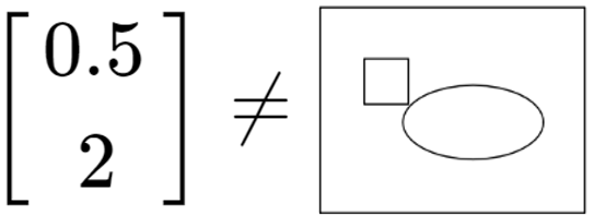
Let’s start with an example that will show us how matrix multiplication transforms data to reveal new insights. Say there’s a population of cats and rats, and we represent them in a dataset. However, the dataset is only able to measure two features: body size, and face length (or more specifically, snout length).

Figure 1: Cat

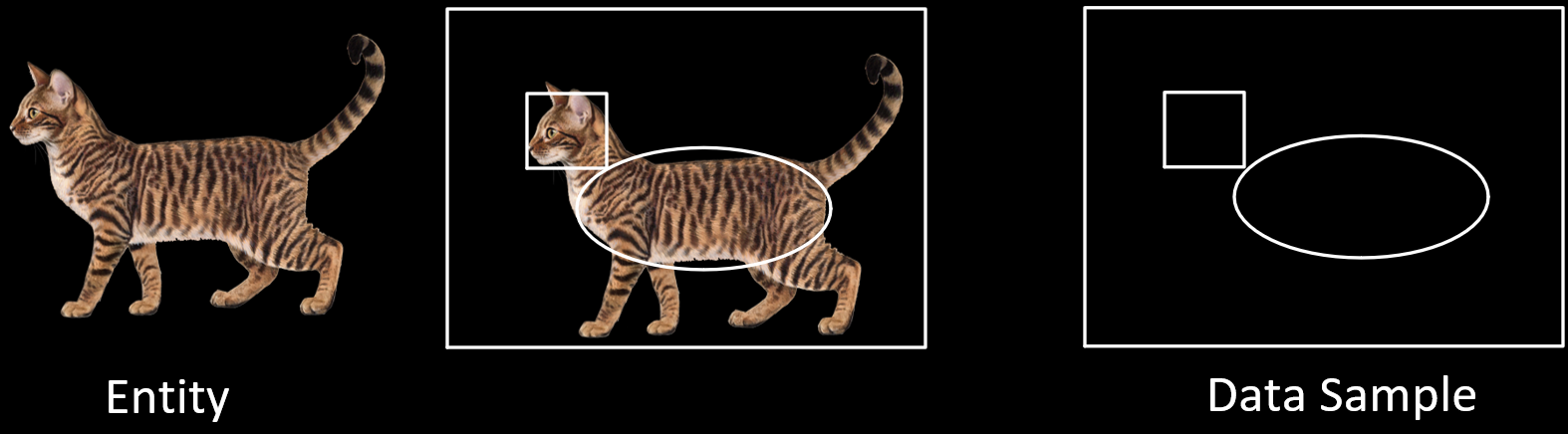
So every entity (a cat or rat) in the population is represented in the dataset as an data sample, which is an abstraction defined only by body size and face length, such that their values are measured in “units”. We can represent the data samples in this dataset as points in a coordinate space, using the two features as axes. The figure below shows the dataset on the left, and its coordinate space representation on the right. The top part shows the data points using numbers, and the bottom part shows how each data point corresponds to a data sample:

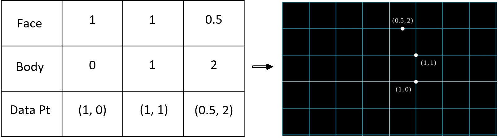
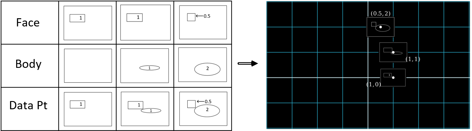
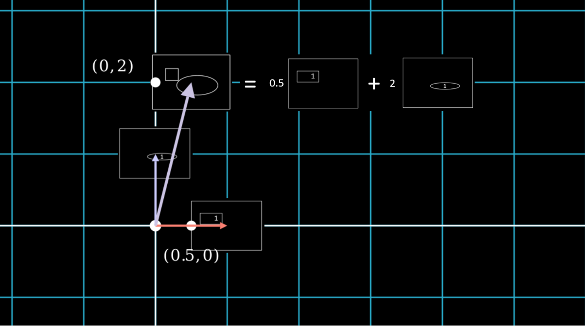
Let’s look at our coordinate space with only the data samples corresponding to unit 1:

Every data point is a combination of the “unit 1” points, which represent and . For instance, the data point (0.5, 2), which represents , is a weighted combination of 0.5 * and 2*

Figure 5: Linear Combination

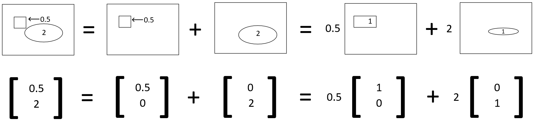
If we see each data point as a vector, then every vector such as is an addition of and , which are basis vectors. Thus (0.5, 2) can also be represented as $\begin{bmatrix} 0.5 \\ 2 \end{bmatrix} = 0.5 \begin{bmatrix} 1 \\ 0 \end{bmatrix} + 2 \begin{bmatrix} 0 \\ 1 \end{bmatrix}$

What is a Change of Basis?

Now, there are other ways we can measure the data samples in this population. Instead of labeling each data sample using the face & body measurements, let’s label each data sample using the following two measurements:

1) How likely it is to be a Cat

2) How likely it is to be a Rat

How do we find the values of these new, and currently unknown, measurements? We can calculate them using our previous known measurements, face & body. For example:

Shorter face + Bigger body = Cat

Longer face + Smaller body = Rat

What are $face_{cat}$ and $body_{cat}$? These are how much each feature is weighted by to calculate the score of “likely to be cat”. The higher the weight, the more that feature is taken into account during calculation. For example, it might be more important to know the body size than the face length when determining if something is a cat or a rat, since cats are usually much bigger than rats, but their faces aren’t always much shorter. Since body size is more important, we’d set $body_{cat} = 1.5 > face_{cat} = 1$. We will reveal how these weights are related to the matrix once we get into the algebra of matrix multiplication in Chapter 1.3.

Each measurement acts as a basis vector used to define each data sample. Because this second set of measurements uses different basis vectors than the set of face & body sizes, it forms a different coordinate space. Since each coordinate space provides a different way to represent the data, let’s call each coordinate space a Model.

The face & body size coordinate space will be called Model 1, and the ‘likely to be’ cat or rat coordinate space be called Model 2. As these two measurement methods are measuring the same data samples, the data samples in Model 1 are present in Model 2, but are now measured by different vectors.

In fact, since we are using Model 1 to calculate the values for Model 2, we will see in Chapter 1.3 that we are applying the dot product on face & body to calculate ‘likely to be cat’. Recall that the steps of matrix multiplication consists of dot products; thus, the calculation of Model 2 is none other than matrix multiplication, which was, for certain matrices, shown here to be a rotation. In these examples, we choose a matrix that, upon multiplication, corresponds to a rotation.

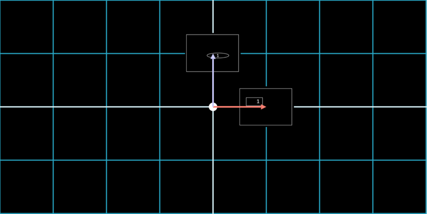
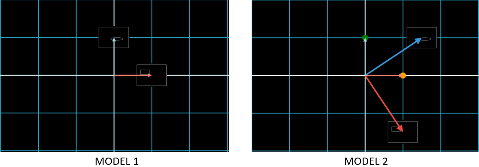
For our examples, say that a vector labels a data sample if it points to it. We know in Model 1 that $\color{#FA8072}{\begin{bmatrix} 1 \\ 0 \end{bmatrix}}$ points to . But does this vector point to the same data sample in Model 2?

Let’s look at the two Models. We’ll use the Orange Dot to denote “likely to be a cat with unit 1”², and use the Green Dot to denote “likely to be a rat with unit 1”.

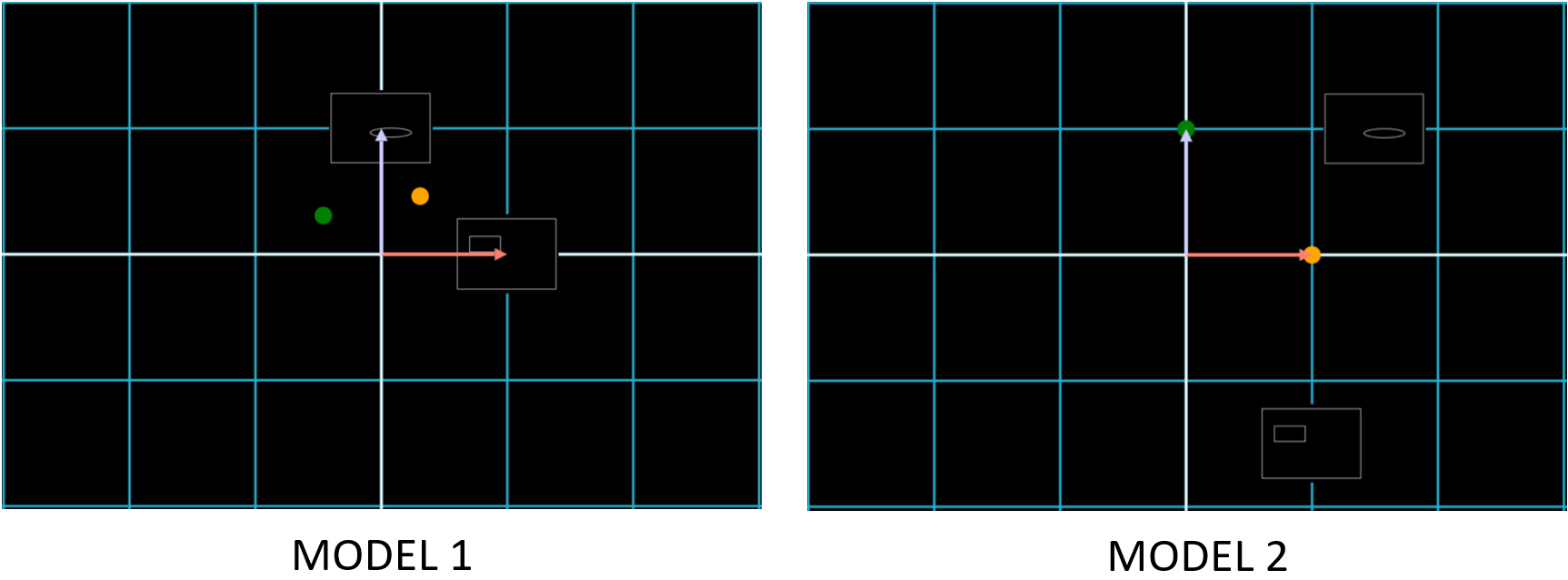
The two $\color{#FA8072}{\begin{bmatrix} 1 \\ 0 \end{bmatrix}}$ in each Model do not label the same data point! Likewise, $\color{#ADD8E6}{\begin{bmatrix} 0 \\ 1 \end{bmatrix}}$ points to in Model 1, but does not point to it in Model 2. Phrasing this a different way makes this idea more intuitive: let’s say that the meaning of a vector is the data sample it points to. $\color{#FA8072}{\begin{bmatrix} 1 \\ 0 \end{bmatrix}}$ no longer has the same meaning in Model 2 as it did in Model 1. This is because the meaning of a vector depends on its basis vectors. In Model 1, $\color{#FA8072}{\begin{bmatrix} 1 \\ 0 \end{bmatrix}}$ pointed to because it’s supposed to mean “has a face with unit 1”. In Model 2, $\color{#FA8072}{\begin{bmatrix} 1 \\ 0 \end{bmatrix}}$ points to Orange Dot because it’s supposed to mean “likely to be a cat with unit 1”.²

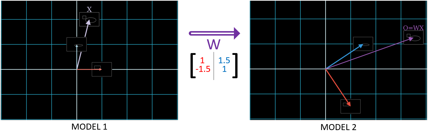
If it’s still not clear why meaning depends on the choice of basis vectors, let’s look at a better example that will help drive home this idea. We know in Model 1 that $\color{#CBC3E3}{\begin{bmatrix} 0.5 \\ 2 \end{bmatrix}}$ labels . But just like before, $\color{#CBC3E3}{\begin{bmatrix} 0.5 \\ 2 \end{bmatrix}}$ in Model 2 does not.

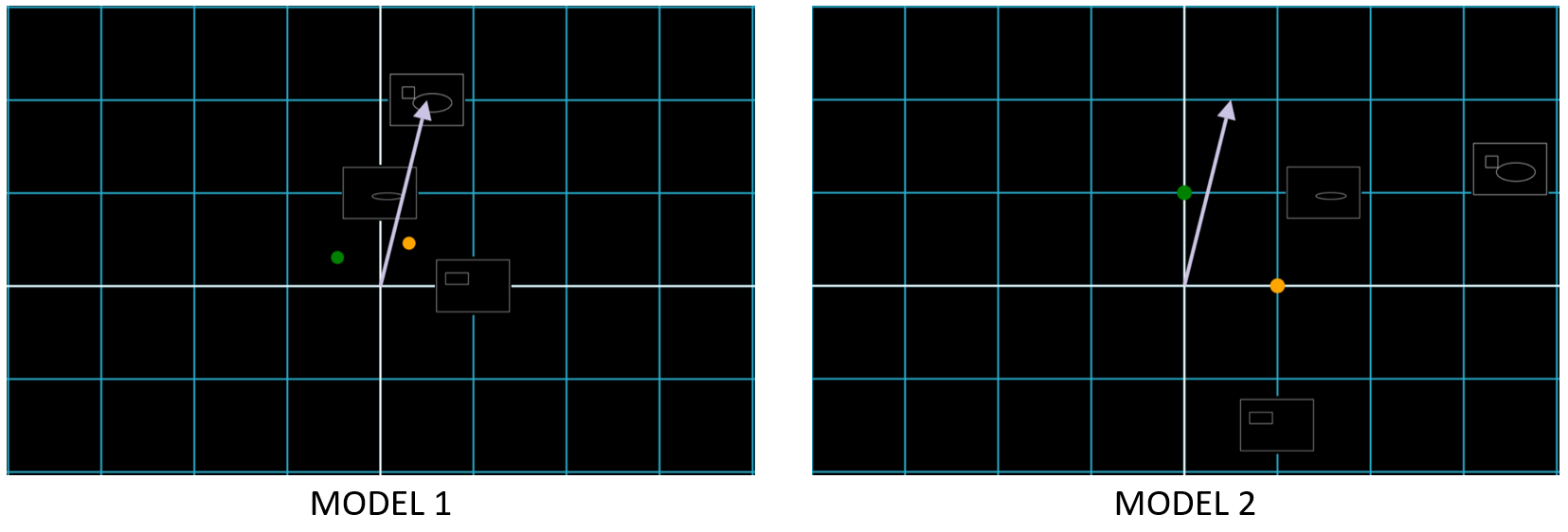
Recall that in Model 1, which uses the face & body sizes as basis vectors, $\color{#CBC3E3}{\begin{bmatrix} 0.5 \\ 2 \end{bmatrix}}$ meant “an entity with a short face (0.5) and a long body (2).” But in Model 2, this vector means “it’s NOT as likely to be a cat (0.5), as it is more likely to be a rat (2)”. The meaning in Model 2 does not point to , because that data sample is likely a cat. Instead, it should point to a data sample that looks more like a rat.

This shows the difference between the data samples coming from the real world, and the model that represents those data samples using labels. $\color{#CBC3E3}{\begin{bmatrix} 0.5 \\ 2 \end{bmatrix}}$ is not itself; it is merely a label of it, and whichever label is used depends on the basis vectors used to define the parts of each label. Note that there is a difference between points, vectors and features. ³

Understanding the difference between a model representation and the actual entity it means (or points to) is crucial for gaining better intuition behind why matrix multiplication reveals hidden information in data sets.⁴

We show below how the features on the two basis vectors in Model 1 are rotated onto two new vectors in Model 2. This is done by matrix multiplication, causing the basis vectors in Model 2 to now point to the Orange Dot and Green Dot; Chapter 1.3 will make it even more clear why matrix multiplication is called a “Change of Basis”.

2mod_vecs

What does Change of Basis have to do with Neural Networks?

Notice that Model 2 demonstrates an idealized, simplified example of what a neural network does- it is making a guess about the data point given to it as input. In fact, one can think of it as a single layer ‘neural network’⁵ such that for the function that calculates the neuron activations:

$$O = \sigma(WX + b)$$

Which, for a data sample, outputs the values it guesses for the 2 classes {cat, rat}, it sets $\sigma = I$, the identity function, and b = 0:

$$O = WX$$

2mod_out

We can see how this matrix relates to weights in a neural network; each column corresponds to outgoing weights of a previous layer neuron, and each row corresponds to incoming weights of a next layer neuron:

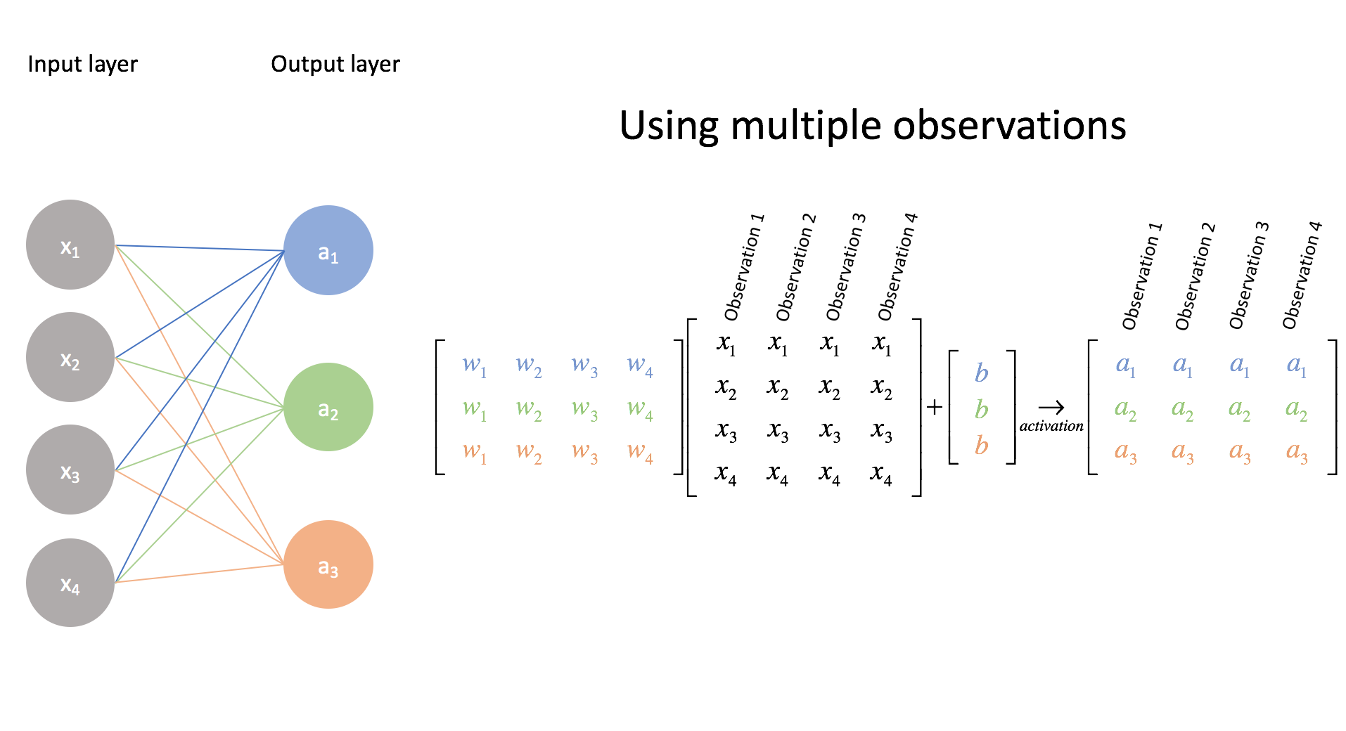
**Image Source: https://www.jeremyjordan.me/intro-to-neural-networks/**

As we see that each of the four neurons on the left act as basis vectors in the previous layer (Model 1), and the three neurons on the right act as basis vectors in the next layer (Model 2), such that the three neurons on the right are a linear combinations of the previous layer neurons and their weights, we come to a very important concept:

Neurons are Basis Vectors in an Activation Space.

Thus, every neuron in a neural network is a measurement on the data. It is possible for a neuron to learn to measure cats, as in the examples shown above, and thus act as a “cat neuron”. This Activation Space is commonly referred to as a Latent Space, and will be a very important concept for describing how a neural networks finds new relationships between data in a dataset.⁶

Going back to the change of basis example above, in Model 2, $\color{#CBC3E3}{X = \begin{bmatrix} 0.5 \\ 2 \end{bmatrix}}$ no longer labels ; it’s labeled by the vector O. How do we calculate what the new label for is? In other words, how do we calculate the values of the vector O = WX by multiplying vector X with matrix W? We will reveal the answer in Chapter 1.3.

With all this in mind, we can say that the goal of the neural network is to find how to accurately measure the data using neuron weights, so they can be taken together into an equation which measures a “goal measurement” such as “how body size and face length determine a cat or a rat”.

NEXT: CHAPTER 1.2

This Chapter is heavily built on 3Blue1Brown’s Essence of Linear Algebra. There are 16 videos, but you only have to focus on five videos: 1 to 3, then 9 and 13. ↩
What does it mean to have 1 unit of “likely a cat?” For our example, we generalize these units to allow any ‘probabilistic’ measurement to be used, as long as having X+1 units means ‘it is more likely to be” than having X units. ↩ ↩²
However, there is a difference between points on a coordinate space and a vector. A vector is mapped onto points in a coordinate space, but it is NOT the point in a coordinate space it is mapped on. Given that it just has length and direction, it can be moved freely anywhere on a coordinate space. The vector’s components are NOT points on a coordinate space, but a way to capture the vector’s length and magnitude in terms of the coordinate space’s basis vectors. This also means that the data point, or feature, that the vector is mapped to can be moved freely anywhere on a coordinate space! What’s important is how features and vectors are relative to other features and vectors in the current coordinate space. ↩
While the vectors are representations of the data sample, the data sample is also a representation of the actual cat entity (by transitivity, both are representation of the entity). Note that the vector is a numerial representation of the data sample, while the data sample is a collection of values which are defined relative to other samples in the population. Information about these collections of relative values is preserved under different Models, and different transformations preserve different information. Because values are defined relative to other values, information about data samples (such as their distribution) are relations, and relations can be thought of as shapes; for instance, a line is a relation between two points, so this line shape describes their relation. This is better explained in Appendix Chapter 1.1. Also note that the only information the neural network knows about the entity comes from the data sample; it can never truly know the entity. ↩
https://ml4a.github.io/ml4a/how_neural_networks_are_trained/ ↩
In this example, the activation function $\sigma$ is the Identity, so the neuron function $O = \sigma(WX + b)$ is linear. But $\sigma$ is usually nonlinear, giving rise to nonlinear functions in latent spaces. ↩