CHAPTER 2.2

CHAPTER 2.2: Conditioning on Features using Orthogonal Projection

(Reading time: 12 minutes)

Now we want to change a feature $n_1$ while keeping the value of another feature $n_2$ the same. Another way to say the value of $n_2$ is “preserved” is to say that we are conditioning on $n_2$. The difficulty in doing this is that each feature vector is made up of the same basis vectors (neurons), so by changing feature $n_1$, you are changing the basis vectors that add up to $n_1$, and since those basis vectors also add up to $n_2$, you are also changing $n_2$.

In other words, a sample lies on a point in a high dimensional latent space of potentially billions of neurons. A feature vector lies along a subspace- a plane¹- within this latent space. Projecting the sample down to this feature subspace (that is, finding its “shadow” or its “distorted reflection” on the plane) measures how much of the feature that sample has.

So when you move a sample from one point to another, the shadow won’t just change on one feature subspace, but another feature subspace. For example, if you are ever stuck in a hall of mirrors, you may find yourself next to two mirrors- one that makes you larger, and one that makes you small. When you move one way, you are not just changing how you look in the “Larger” mirror, but also how you look in the “smaller” mirror.²

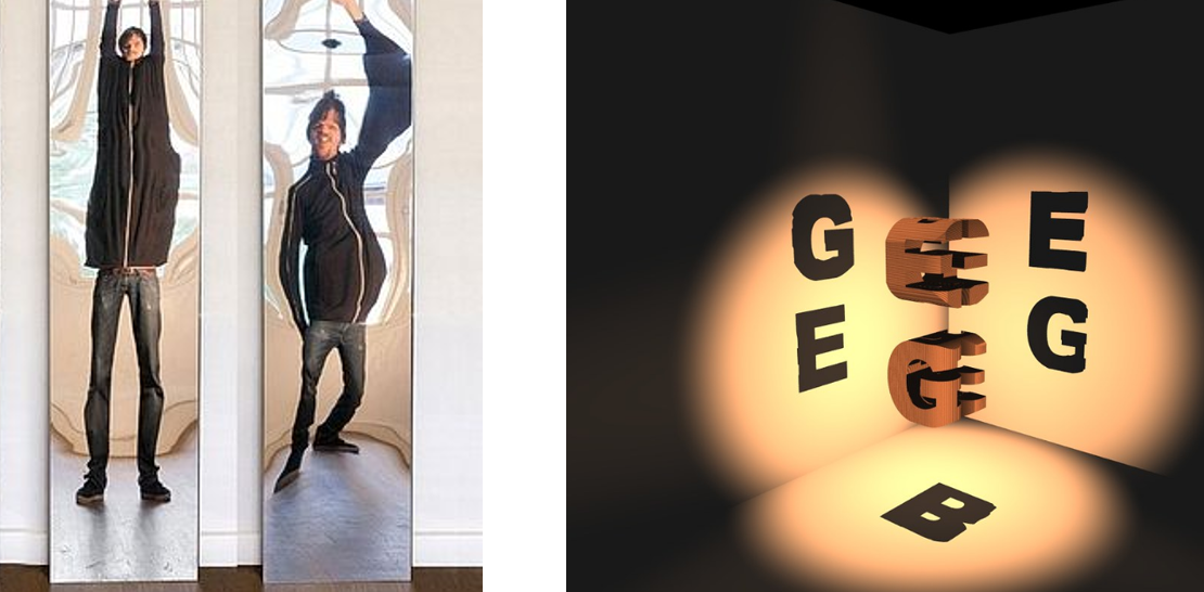
Sources: https://www.thisiswhyimbroke.com/uk/warping-mirrors/
https://www.flickr.com/photos/51339555@N02/5252365635

When changing one feature vector affects another, the feature vectors are entangled. However, it is possible to find a new feature vector that will cast the new desired shadow on $n_1$ but also tries not to change the existing shadow projected onto $n_2$. This procedure will find a vector disentangled to $n_2$.

Thus, we will have to find a new vector to add to our sample $z$.

Changing a Feature while Conditioning on Another Feature that’s on a Basis Vector

In the previous section, we already saw a case where the feature we want to change, $y$, is on the basis vector.

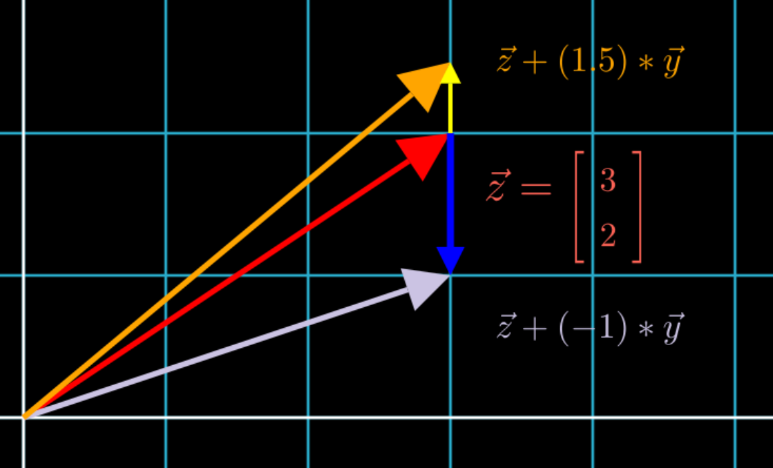
Notice that all the new samples have the same value: x = 3. So changing y doesn’t change x. Also note that the x-axis basis vector and the y-axis basis vector are at a 90 degree angle to each other. This should give a hint as to where we’re going with this.

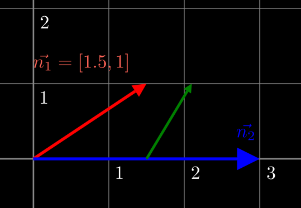
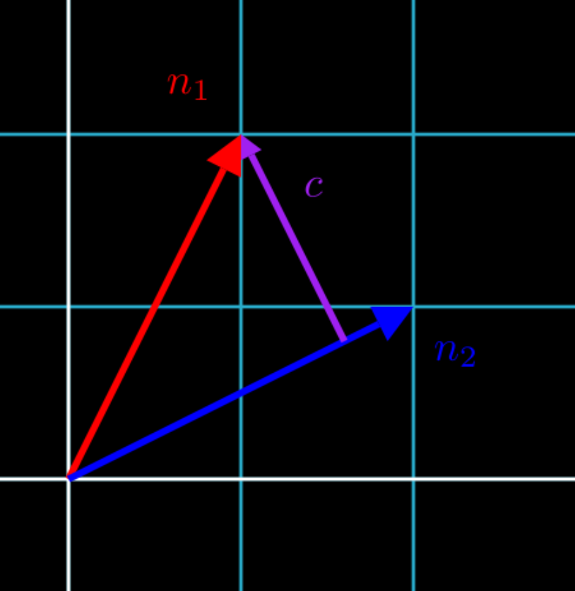
Let’s start with the case where sample $z = [3, 1]$, and the feature $n_1 = [1.5, 1]$ we want to change is not on a basis vector, but the feature $n_2$ whose value of a sample we want to keep is on a basis vector. To find a new feature vector $c$ to add to $z$, we want $c$ to keep $n_2 = 3$, but want the other parts of $c$ be as close to $n_1$ as possible.

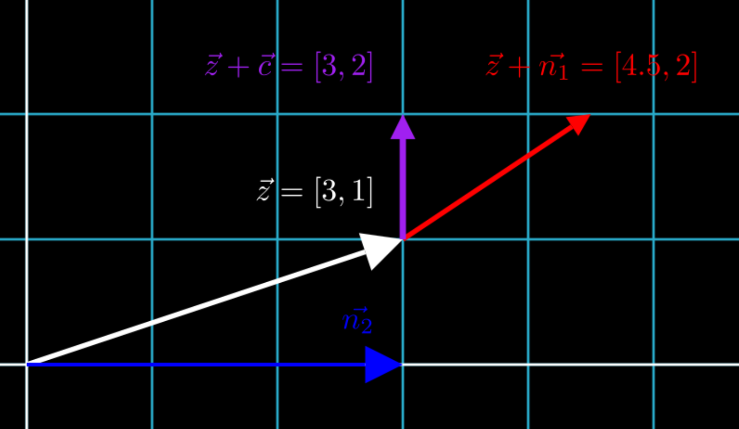
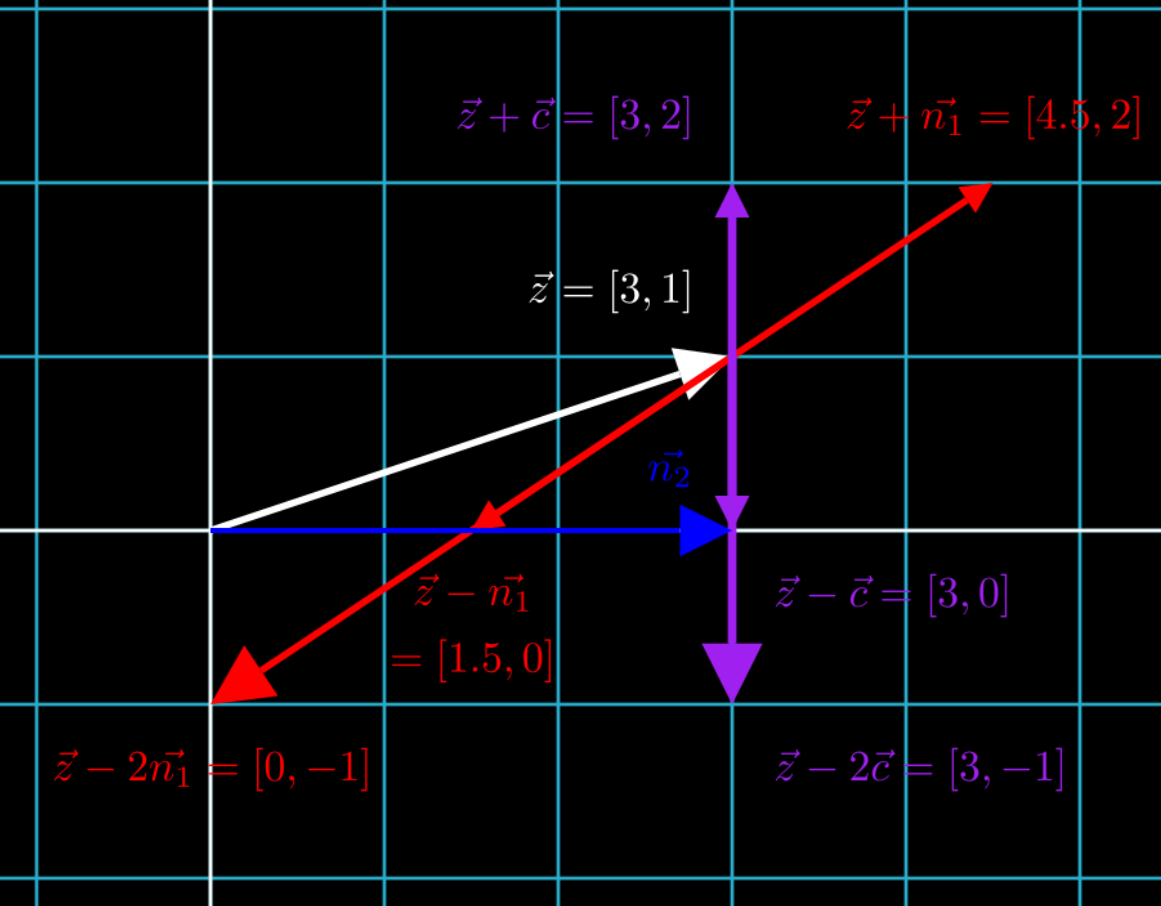
In the figure above, we see that vector $z + c$ keeps as much of $n_1 = [1.5, 1]$ as possible- that is, it still lies at $y = 1 + 1 = 2$ just like $z + n_1$, but also keeps $n_2 = 3$, in contrast to $z + n_1$, which moves $n_2$ to 4.5.

Let’s reframe these vectors $n_1$, $n_2$ and $c$ by moving them to the origin, and independent of $z$. Given that $c$ is a vector and thus is actually just has no true coordinates, just an object with length and direction ³, we can move it to the right.

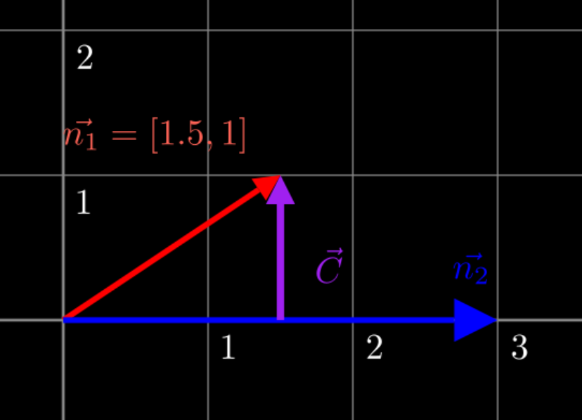
Why does vector $c$ not change the value of $y=1$? Because vector $c$ is orthogonal to $n_2$, meaning they are at a 90 degree angle, where they intersect at $n_2 = 1$. If it was not orthogonal, it would veer away from $n_2 = 1$, such as shown in the example below, where a non-orthogonal vector leads to $n_2 = 2.1$.

How do we calculate the value of this orthogonal vector $c$?

In this case, because $n_1$ is a sum of $n_2$ and $y$, and $n_2$ is a basis vector, when we “remove” $n_2$ from $n_1$, we are just left with $y$, so we can move in the y-direction by simply changing the y-coordinate value. Notice that vector $c$ is parallel to the y-direction, and thus moving along $c$ means moving along $y$.

Even so, let’s actually calculate vector $c$ in terms of $v$ and $x$, because this calculation can be generalized to the case where the feature we want to change is not on a basis vector.

First, let’s describe what we want, and then translate that description into mathematics. Overall, we want:

“A vector which preserves the values of how much of $n_2$ is used to get vector $n_1$”.

Let’s break this down into parts. To preserve the values of “how much of $n_2$ is used to get vector $n_1$”, we need to represent this phrase in terms of vectors. Recall from Chapter 1 that this can be done using the dot product, which projects one vector onto another, outputting a scalar that says “how much of $n_2$ is used to get vector $n_1$”.

So if $\vec{n_1} = \color{red}{\begin{bmatrix} 1.5 \\ 1 \end{bmatrix}}$, then $\vec{n_1} \cdot \vec{n_2} = 1.5$

Then, we scale the $n_2$ basis vector by $\vec{n_1} \cdot \vec{n_2}$ by doing:

\[(\vec{n_1} \cdot \vec{n_2}) * \vec{n_2}\]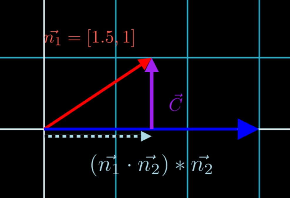

In Figure 2.3 above, we have found the vector, shown in light blue, that represents “how much of $n_2$ is used to get vector $n_1$”. Now to “preserve” this value of $(\vec{n_1} \cdot \vec{n_2})$ while changing as much of $n_1$ as we can, we have to calculate the vector $c$ that’s “orthogonal” to $(\vec{n_1} \cdot \vec{n_2}) * \vec{n_2}$. Since $c$ starts at the head of $(\vec{n_1} \cdot \vec{n_2})$ and ends at the head of $\vec{n_1}$, in vector addition, that translates to:

\[\vec{n_1} = (\vec{n_1} \cdot \vec{n_2}) * \vec{n_2} + \vec{c}\]

Solving for $\vec{c}$, we obtain:

\[\vec{c} = \vec{n_1} - (\vec{n_1} \cdot \vec{n_2}) * \vec{n_2}\]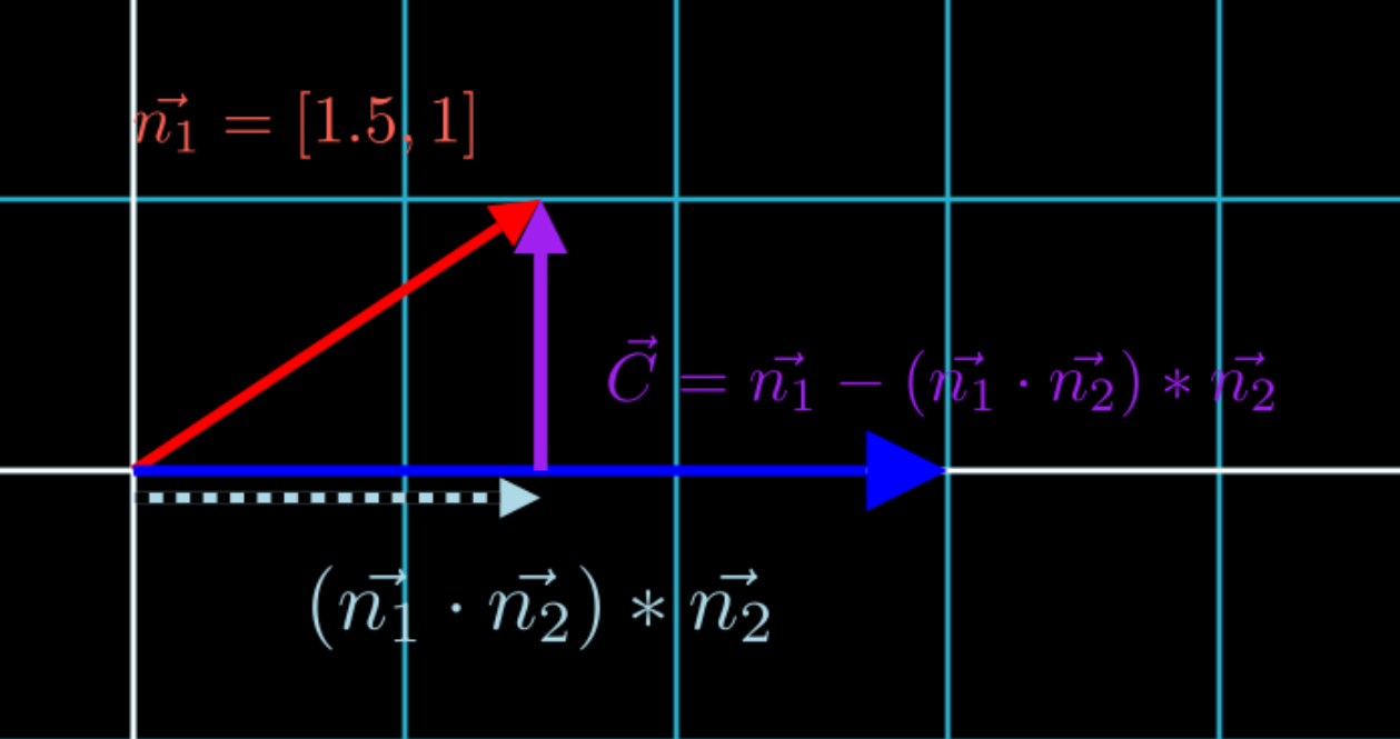

And so any sample along:

\[\vec{z} + \alpha * \vec{c}\]

Would be a sample that fits our criteria. No matter what value of $\alpha$ we use, we see that $\alpha * \vec{c}$ is as close to $\alpha * \vec{n_1}$ as possible while keeping $n_2 = 3$:

Let’s further analyze this by plugging in specific values.

\[\vec{c} = \vec{n_1} - (\vec{n_1} \cdot \vec{n_2}) * \vec{n_2} = [1.5, 1] - (1.5) * [1, 0] = [1.5 - 1.5, 1] = [0,1]\]

We see that this subtraction is actually “removing” parts of $n_2$ from $n_1$ to obtain $c$, which is just $y$ in this case. But what if $n_2$ was not on the basis, and thus was not orthogonal to $y$ or any other basis vector? We’ll see soon that the calculation follows the same logic as the one for C that we did just now.

Changing a Feature while Conditioning on Another Feature IN GENERAL

Now let’s say we have a feature vector $n_1 = (1,2)$ and feature vector $n_2 = (2,1)$. Based on the previous section, we want to find samples along the purple line in the figure below:

Recall from the previous section that if we wanted to vary the features of a vector $n_1$, but wanted to keep the value at vector $n_2$, we used the equation:

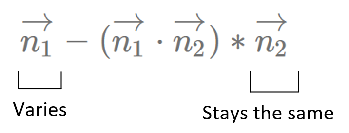
Here, let’s use a similar version of the equation, but we will slightly modify the dot product projection to include a denominator term, as shown below:

\[\frac{(\vec{n_1} \cdot \vec{n_2}) }{(\vec{n_2} \cdot \vec{n_2}) } * \vec{n_2}\]

The reason this denominator was not needed in the previous example was because it measures the length of the vector being projected onto; in that case, vector $\vec{n_2}$ was a basis vector with a length of 1, so this term simplified to just the numerator.

Then our equation for finding $c$ becomes:

\[\vec{c} = \vec{n_1} - \frac{(\vec{n_1} \cdot \vec{n_2}) }{(\vec{n_2} \cdot \vec{n_2}) } * \vec{n_2} * \vec{n_2}\]

This is the equation for orthogonal projection, which will find the vector scaled on $n_2$ that’s closest to $n_1$. The proof for the equation is linked in the footnotes.⁴

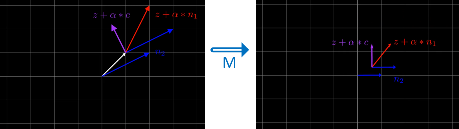
But why is this the case? We don’t immediately see how this “preserves” the other features of $n_2$, like we saw how $n_2 = 3$ was preserved by going orthogonal to it in the previous example. Intuitively, it becomes more obvious when we perform a change of basis to measure our data in terms of $n_2$:

Click here to see the animation

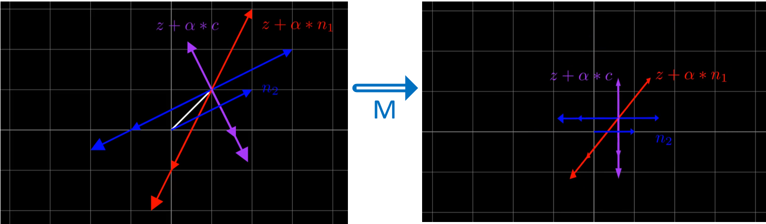
As in the previous example, $c$ tries to be as “close to” $n_1$ as possible, while still preserving the value at $n_2$. This is even more evident when there are multiple samples of $\alpha = -1$ and $\alpha = -1.5$:

Click here to see the animation

The matrix used here is calculated in the same way that that matrix for the change of basis in the previous section was calculated. Note that for the vector orthogonal to $n_2$, we are using $c = [-0.6, 1.2]$:

$$ M = \begin{bmatrix} 2 & -0.6 \\ 1 & 1.2 \end{bmatrix}^{-1} = \begin{bmatrix} 0.4 & 0.2 \\ -0.3333 & 0.6667 \end{bmatrix} $$

When the change of basis is performed, we see that all the values at $z + \alpha * c$ are orthogonal to $n_2$. The values at $z + \alpha * n_1$ are $z + \alpha * c$ share similar values on the new y-axis, $c$.

Now, we see that the removal of the projection onto $n_2 = [2, 1]$ from $n_1 = [1, 2]$ will leave more than just the basis vector, as in the original coordinate space, $c = [-0.6, 1.2]$ is not a basis vector.

When there are more than two dimensions, this removal of the projection will be even more non-trivial. One can say that since $(\vec{n_1} \cdot \vec{n_2}) * \vec{n_2}$ says “how much of $n_2$ is used to calculate $n_1$”, that it’s the “effect of $n_2$ on $n_1$”. So by removing it, we are removing the effect of $n_2$ on $n_1$.

Changing a feature while keeping MULTIPLE features the same

To do so, the paper says: “If there are multiple attributes to be conditioned on, we subtract the projection from the primal direction onto the plane constructed by all conditioned directions.” ⁵

“Attribute” is synonomous with “feature”, and “direction” is synonomous with “feature vector”. The “primal direction” is the feature we want to change, while all other features are kept the same. But how do we know which features these are? We can’t keep ALL the features the same.

Essentially, this manipulation cannot make ALL features stay the same. We must know beforehand which features we want to stay the same, and which features we want to vary. Then, we will condition on the features we want to stay the same. For example, we can change age while conditioning on hair style, eye color, and ear size. We will only aim to keep those 3 features the same; all other features may vary.

Finally, the “plane constructed by all conditioned directions” is the subspace spanned by all the feature vectors we want to condition on. ⁶

We are done with explaining how orthogonal projection is used in InterFaceGAN. Next, we will describe how hyperplanes are used to obtain “semantic scores” for how close a sample is to a feature boundary.

NEXT: CHAPTER 2.3

If the activation function $\sigma$ is linear, the neuron function $O = \sigma(WX + b)$ is linear. But $\sigma$ is usually nonlinear, giving rise to nonlinear functions in latent spaces. Thus, instead of projecting down to planes, projections would be done down to surfaces. ↩
By pure speculation, this may some link to how concepts are organized, and how concepts can be related to one another by analogy. An analogy relates an “abstraction” of concepts- such as abstracting the Hero’s Journey in The Hunger Games and in Harry Potter. There is some sort of semantic (but possibly superficial, and thus meaningless) similarity between Projection and Abstraction. Abstractions also occur in dreams, where a memory of an angry neighbor yelling at his lawn may be substituted with the dream of an angry teacher yelling at his lawn, which has never occurred in real life. Now projecting down to different abstractions would mean if the way a sample is mapped to one abstraction framework is changed, then the way it’s mapped to another abstraction framework is also changed. So say you’re trying to think of a way to create a novel concept by slightly tweaking an existing concept. The difficulty is that some abstraction frameworks cannot be changed in order to preserve the concept itself. For example, you want to write a story that has the same “beats” as Star Wars. Now your story contains an abstraction of “Star Wars”, and also an abstraction on “The Hero’s Journey”. If you want to get rid of “The Call to Adventure”, you would also shake your story away from “The Hero’s Journey”. (NOTE: This is not a good example, so further thought will be put into it). In any case, there is no evidence so far that existing neural networks relate “abstraction” with “projection”, nor is there evidence suggesting this is a concept that can be used for building new methods, but it is an interesting idea to test out to see if there is potential. ↩
There is a difference between points on a coordinate space and a vector. A vector is mapped onto points in a coordinate space, but it is NOT the point in a coordinate space it is mapped on. Given that it just has length and direction, it can be moved freely anywhere on a coordinate space. The vector’s components are NOT points on a coordinate space, but a way to capture the vector’s length and magnitude in terms of the coordinate space’s basis vectors. This also means that the data point, or feature, that the vector is mapped to can be moved freely anywhere on a coordinate space! What’s important is how features and vectors are relative to other features and vectors in the current coordinate space. ↩
Proof for the orthogonal projection equation. Find it using ctrl+f “Recipe: Orthogonal projection onto a line”. Another resource is here. ↩
Yujun Shen, Jinjin Gu, Xiaoou Tang, and Bolei Zhou. Interpreting the latent space of GANs for semantic face editing. CoRR, abs/1907.10786, 2019. ↩
A spanning set is just “the collection of all linear combinations of vectors.”; these vectors ‘span’ the space that contains all their linear combinations. However, a basis set requires a linearly independent spanning set. Finally, not all linearly independent sets are orthogonal, unless all the vectors in the set are nonzero or orthonormal. ↩