CHAPTER 1.3

CHAPTER 1.3: Why is the Dot Product used in Matrix Multiplication?

(Reading time: 12 minutes)

Let’s re-visit the problem of finding the value of $O$. In other words, how do we find the new label of in Model 2?

2mod_vecs

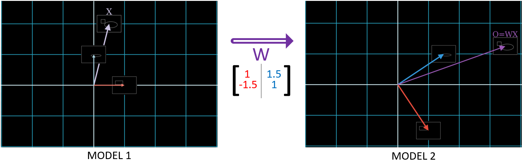
In a linear algebra class, one learns that this can be done using matrix multiplication. But why does the algebraic procedure of matrix multiplication work? Why does the first step specifically use the dot product of the first row and the input vector? What even is a dot product?

And What Do Dot Products have to do with Measurement?

Let’s figure this out by first understanding what we need to know to calculate the values of $O$ that represents data sample . All data samples in Model 2 are represented by two measurements:

1) How likely it is to be a Cat

2) How likely it is to be a Rat $$O = \def\a{\color{orange}{Cat}} \def\b{\color{green}{Rat}} \begin{bmatrix} \a \\ \b \end{bmatrix}$$

So if we want to find the value of $O$, we need to calculate these two values. Recall in the previous section that we were able to calculate the value of “how likely to be cat” using the values of “face length” and “body size”:

Shorter face + Bigger body = Likely a Cat

$\color{red}{face_{cat}} * 0.5 + \color{blue}{body_{cat}} * 2$ = the value 0.5(face_cat)+2(body_cat) on the cat axes

Notice how this resembles the following dot product: ¹

$$ \def\a{\color{red}{face_{cat}}} \def\b{\color{blue}{body_{cat}}} \begin{bmatrix} \a & \b \end{bmatrix} \cdot \begin{bmatrix} 0.5 \\ 2 \end{bmatrix} = \color{red}{face_{cat}} * 0.5 + \color{blue}{body_{cat}} * 2$$

Not only that, but it resembles the first step of matrix multiplication:

$$ \def\a{\color{red}{face_{cat}}} \def\b{\color{blue}{body_{cat}}} \begin{bmatrix} \a & \b \\ ? & ? \end{bmatrix} \begin{bmatrix} 0.5 \\ 2 \end{bmatrix} = \begin{bmatrix} \a * 0.5 + \b * 2 \\ ?\end{bmatrix} $$

In fact, the matrix on the left is none other than $W$ from the figure above, which is used in the equation $O = WX$.

\[\def\a{\color{red}{1}} \def\b{\color{blue}{1.5}} \def\c{\color{red}{-1.5}} \def\d{\color{blue}{1}} \begin{bmatrix} \a & \b \\ \c & \d \end{bmatrix} = \def\a{\color{red}{face_{cat}}} \def\b{\color{blue}{body_{cat}}} \begin{bmatrix} \a & \b \\ ? & ? \end{bmatrix}\]

We mentioned that $face_{cat}$ and $body_{cat}$ are weights that denote how important each feature is in the calculation. For example, if body size is more important, we’d set $body_{cat} = 1.5 > face_{cat} = 1$.

But what does this dot product mean in terms of our dataset? To make its meaning easier to understand, let $face_{cat}=4$, and let’s ignore the second term by setting $body_{cat} = ?$

\[\color{red}{W}\color{#CBC3E3}{X} = \color{orange}{O}\]

$$ \def\a{\color{red}{(face_{cat}=4)}} \def\b{\color{#CBC3E3}{0.5}} \def\c{\color{red}{4}} \def\d{\color{orange}{2}} \begin{bmatrix} \a & ? \\ ? & ? \end{bmatrix} \begin{bmatrix} \b \\ ? \end{bmatrix} = \begin{bmatrix} \c * \b = \d \\ ?\end{bmatrix} $$

0.5 units of face length → 2 units of 'likely to be cat'

In other words, “for every face length of unit 1, there are 4 units of cat”. Thus, for half a unit of face length, we have half of the proportionate amount of cat, which is 2. Doesn’t this sound familiar, like unit conversion?

For every 1 meter, there are 3.28 feet. So if an entity is 2 meters long:

$$ \def\a{\color{red}{(meter_{feet}=3.28)}} \def\b{\color{#CBC3E3}{2}} \def\c{\color{red}{3.28}} \def\d{\color{orange}{6.56}} \begin{bmatrix} \a \end{bmatrix} \begin{bmatrix} \b \end{bmatrix} = \begin{bmatrix} \c * \b = \d \end{bmatrix} $$

2 units of meter → 6.56 units of feet

Indeed, one dot product step is analogous to 1D matrix multiplication; so two dot product steps would be analogous to 2D matrix multiplication. At last, we realize that matrix multiplication, or “Change of Basis”, is none other than unit conversion multiplication, or “Change of Units”. That is, $O$ refers to the same quantity that $X$ refers to, except the two vectors measure it using different units.²

But in contrast to the 1D “meter to feet” example, the “face and body to cat” example uses two measurements to find the value of cat. Matrix multiplication allows for a change of multiple units, or multiple dimensions. The weight matrix $W$ is analogous to the conversion factor.

In summary:

1) A Dot Product is used to convert multiple units into a new unit

2) Multiple dot products are used in Matrix Multiplication to find multiple new units

Just like how each row of $X$ measures the same entity but using a different unit (a basis vector of Model 1), each row of $O$ uses a different unit (a basis vector of Model 2) to measure the same entity, and each is calculated using the known measurements from $X$.

Since each new measurement is calculated using the same input, but with different conversion factors, each new value of $O$ is calculated using the same input vector $X$, but with different rows of $W$. ³

What are the Columns of a Matrix?

We now explained what the rows of $W$ are. But what are its columns? And how does this tie into the geometric representation of matrix multiplication, as we see in the figure above? Let’s match terms in these equations to their geometric representation:

In Model 1, $\def\a{\color{#FA8072}{1}} \def\c{\color{#FA8072}{0}} \begin{bmatrix} \a \\ \c \end{bmatrix}$ labels . In Model 2, $\def\a{\color{red}{1}} \def\c{\color{red}{-1.5}} \begin{bmatrix} \a \\ \c \end{bmatrix}$ labels .

Thus, $\def\a{\color{red}{1}} \def\c{\color{red}{-1.5}} \begin{bmatrix} \a \\ \c \end{bmatrix}$ is where the data sample previously labeled by the basis vector $\def\a{\color{#FA8072}{1}} \def\c{\color{#FA8072}{0}} \begin{bmatrix} \a \\ \c \end{bmatrix}$ is sent.

Notice that $\def\a{\color{red}{1}} \def\c{\color{red}{-1.5}} \begin{bmatrix} \a \\ \c \end{bmatrix}$ is the first column of $W$. And $\color{red}{face_{cat}}$ = 1 is the Cat coordinate of the vector $\def\a{\color{red}{face_{cat}=1}} \def\c{\color{red}{-1.5}} \begin{bmatrix} \a \\ \c \end{bmatrix}$ in Model 2. Given the fact that the vertical axis of Model 2 denotes “likely to be rat”, it’s pretty clear that the second row of this vector is $face_{Rat}$, which is how much the face length is weighed by to calculate the value of the Rat coordinate.

Therefore, $\def\a{\color{red}{face_{cat}=1}} \def\c{\color{red}{face_{Rat}=-1.5}} \begin{bmatrix} \a \\ \c \end{bmatrix}$, the first column of $W$, and the Model 2 vector labeling , contains the conversion factors for each of the basis vectors $\{ \color{orange}{cat}, \color{green}{Rat} \}$ of Model 2, in terms of only $\color{red}{face}$.⁴

Likewise, $\def\a{\color{blue}{body_{cat}=1.5}} \def\c{\color{blue}{body_{Rat}=-1}} \begin{bmatrix} \a \\ \c \end{bmatrix}$, the second column of $W$, and the Model 2 vector labeling , contains the conversion factors for each of the basis vectors $\{ \color{orange}{cat}, \color{green}{Rat} \}$ of Model 2, in terms of only $\color{blue}{body}$.

\[\def\a{\color{red}{face_{cat}}} \def\b{\color{blue}{body_{cat}}} \def\c{\color{red}{face_{Rat}}} \def\d{\color{blue}{body_{Rat}}} \color{purple}{W} = \begin{bmatrix} \a & \b \\ \c & \d \end{bmatrix}\]

If we multiply this by the basis vector in Model 1 that labels , we see it uses ONLY the conversion units for $face$, and none of the conversion units for $body$. This is because this data sample has no body, so it would not use $body$ in its calculation for $cat$ and $rat$ at all. The same goes for the other basis vector in Model 1.

\[\def\a{\color{red}{face_{cat}}} \def\b{\color{blue}{body_{cat}}} \def\c{\color{red}{face_{Rat}}} \def\d{\color{blue}{body_{Rat}}} \begin{bmatrix} \a & \b \\ \c & \d \end{bmatrix} \begin{bmatrix} 1 \\ 0 \end{bmatrix} = \begin{bmatrix} 1 * \a + 0* \b \\ 1 * \c + 0* \d \end{bmatrix} = \begin{bmatrix} \a \\ \c \end{bmatrix}\]

So we arrived at several conclusions:

1) Because Model 2 uses the old measurements of Model 1 to calculate its new measurements, the matrix $W$ contains the weights needed to determine how important each old measurement is for each new measurement

2) Each row of the matrix contains weights to calculate one new measurement in $O$

3) Each column of the matrix contains weights for how one OLD measurement in $X$ is used

4) The dot product is applied between every row of the matrix and the input vector because the same input vector uses different weights of the old measurements in $X$ for every new measurement in $O$

Using a Different Matrix from the Example at the Top

It is important to know that not all matrices are good at their job. The matrix $W$ we have been using is not a good way to calculate “cat” and “Rat”, though it does convey a right rotation, which makes it intuitively easy to see how the basis vectors change between Models:

\[\def\a{\color{red}{1}} \def\b{\color{blue}{1.5}} \def\c{\color{red}{-1.5}} \def\d{\color{blue}{1}} \begin{bmatrix} \a & \b \\ \c & \d \end{bmatrix}\]

Note that it uses $\color{red}{face_{cat}=1}$ and $\color{blue}{body_{cat}=1.5}$. Although $\vert body_{cat} \vert > \vert face_{cat} \vert$, with $\vert \vert$ meaning the value of the weights regardless of sign meets this condition, we would still like longer faces to mean the data sample is less likely a cat. This means we have to penalize bigger values of $face_{cat}$ by choosing a negative value for $face_{cat}$. Likewise, a data sample with a bigger body is less likely to be a rat, so we should also choose a negative value for $body_{Rat}$. The following matrix meets our desired criteria, so we will use it in our examples from now on:

\[\def\a{\color{red}{-2}} \def\b{\color{blue}{2.5}} \def\c{\color{red}{2.5}} \def\d{\color{blue}{-2}} \begin{bmatrix} \a & \b \\ \c & \d \end{bmatrix}\]

What does a negative conversion factor mean?

“A face length of unit 1 denotes that it’s -2 units ‘likely to be cat”

Or in other words, “A face length of unit 1 denotes that it’s 2 units NOT ‘likely to be cat”

Analogies between X=IX and O=WX

We have been thinking of $W$ as a conversion matrix, such that its columns are the basis vectors of Model 2. But how are the basis vectors in Model 1 represented in these equations? Let’s try to put them in columns to see what we get.

\[\def\a{\color{red}{1}} \def\b{\color{blue}{0}} \def\c{\color{red}{0}} \def\d{\color{blue}{1}} \begin{bmatrix} \a & \b \\ \c & \d \end{bmatrix}\]

The basis vectors in Model 1 form $I$, the identity matrix! Multiplying $I$ with any vector leaves that vector unchanged: $X = IX$

We see that $IX$ in Model 1 is analogous to $WX$ in Model 2:

\[IX = \def\a{\color{red}{1}} \def\b{\color{blue}{0}} \def\c{\color{red}{0}} \def\d{\color{blue}{1}} \begin{bmatrix} \a & \b \\ \c & \d \end{bmatrix} \begin{bmatrix} 0.5 \\ 2 \end{bmatrix} = X\] \[WX = \def\a{\color{red}{-2}} \def\b{\color{blue}{2.5}} \def\c{\color{red}{2.5}} \def\d{\color{blue}{-2}} \begin{bmatrix} \a & \b \\ \c & \d \end{bmatrix} \begin{bmatrix} 0.5 \\ 2 \end{bmatrix} = O\]

Note that the basis vectors of Model 1 in $I$ are NOT the rows of I, but the columns. This can be easy to mix up because I is a symmetric matrix, so the $i^{th}$ row equals the $i^{th}$ column.

The first column in each of the matrices labels , and the second column labels . Each value in X is a quantity specifying the values of and ; each value can also be thought of as an instruction on how many units of that basis vector to use. Let’s go through the multiplications of $IX$ and $WX$ side by side to see how different they are when they use different basis vectors.

Matrix Multiplication Visually Explained: Step-By-Step

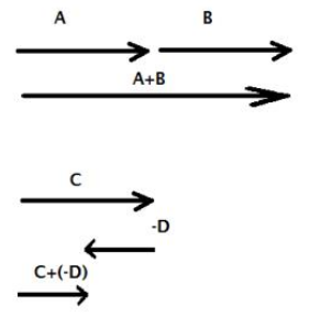
To understand matrix multiplication when it comes to adding the projections onto a basis vector, let’s review 1D vector addition. Given vectors $A + B$, the reason why we add the tail of $B$ to the head of $A$ is because we can think of the tail to head of a vector as being a quantity on a 1D number line. Now for $C + (-1)D$, we are subtracting this quantity:

**Image Source: https://www.slideserve.com/arden/vector-addition-and-subtraction**

Now we’re ready to go through each step of matrix multiplication in an intuitive manner.

(To enlarge each image, right-click and ‘Open image in new tab’. Future updates will allow the image to be enlarged by clicking on it.)

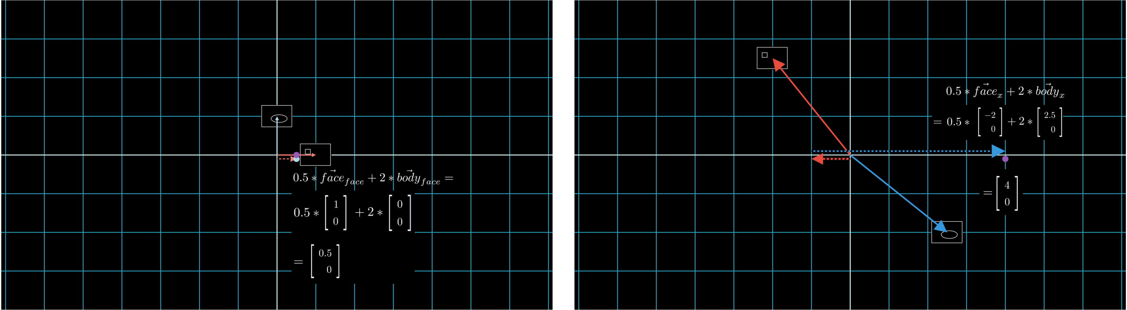
Recall above that we want to find the value of $O$ in Model 2, which is analogous to finding $X$ in Model 1:

In the figures below, on the left side, we’ll be showing matrix multiplication in Model 1, which uses $\def\a{\color{red}{1}} \def\b{\color{blue}{0}} \def\c{\color{red}{0}} \def\d{\color{blue}{1}} \begin{bmatrix} \a & \b \\ \c & \d \end{bmatrix}$ to define its basis vectors.

On the right side, we’ll be showing matrix multiplication in Model 1, which uses $\def\a{\color{red}{-2}} \def\b{\color{blue}{2.5}} \def\c{\color{red}{2.5}} \def\d{\color{blue}{-2}} \begin{bmatrix} \a & \b \\ \c & \d \end{bmatrix}$ to define its basis vectors. We’ll see how the steps in each Model are analogous to each other.

First, we break down the steps of the first dot product, corresponding to the Cat coordinate, involving the first row of the matrices. Let’s find what a and b correspond to in each Model.

[ STEP 1 ] First row of matrix: $\def\a{\color{red}{a}} \def\b{\color{blue}{b}} \begin{bmatrix} \a & \b \end{bmatrix}$

step1

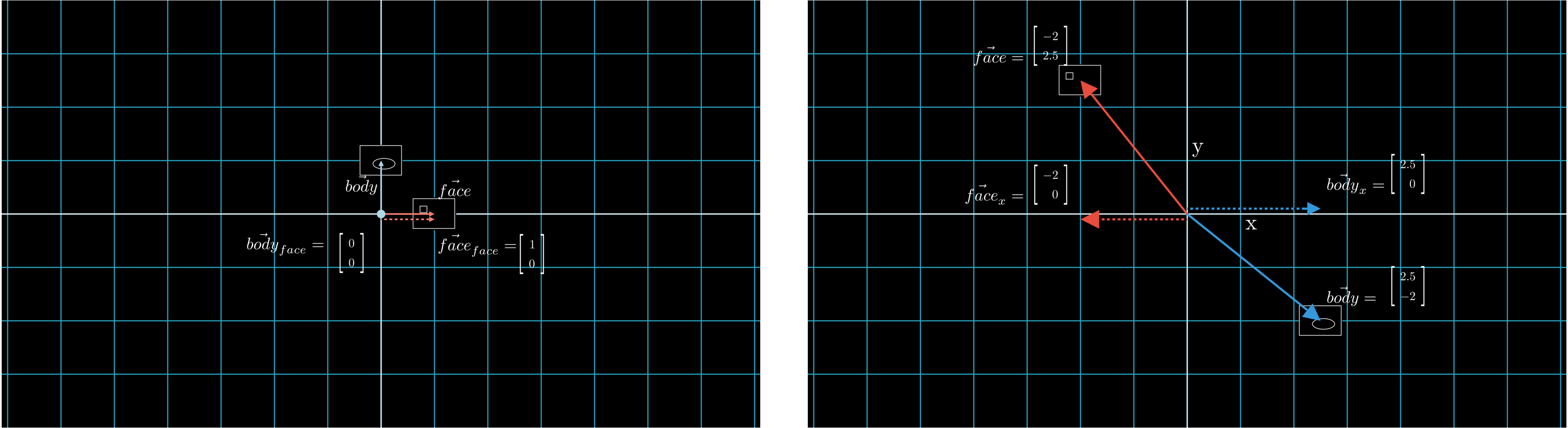
As we see above, the dotted lines are what a and b correspond to in each Model:

$I$: $\def\a{\color{red}{1}} \def\b{\color{blue}{0}} \begin{bmatrix} \a & \b \\ ? & ? \end{bmatrix}$

$W$: $\def\a{\color{red}{-2}} \def\b{\color{blue}{2.5}} \def\c{\color{red}{2.5}} \def\d{\color{blue}{-2}} \begin{bmatrix} \a & \b \\ ? & ? \end{bmatrix}$

[ STEP 2 ] Scale by $X$: $\def\a{\color{red}{a}} \def\b{\color{blue}{b}} \begin{bmatrix} \a & \b \end{bmatrix} \begin{bmatrix} x_1 \\ x_2 \end{bmatrix} --> \color{red}{a} * x_{1}\qquad \color{blue}{b} * x_2$

step2

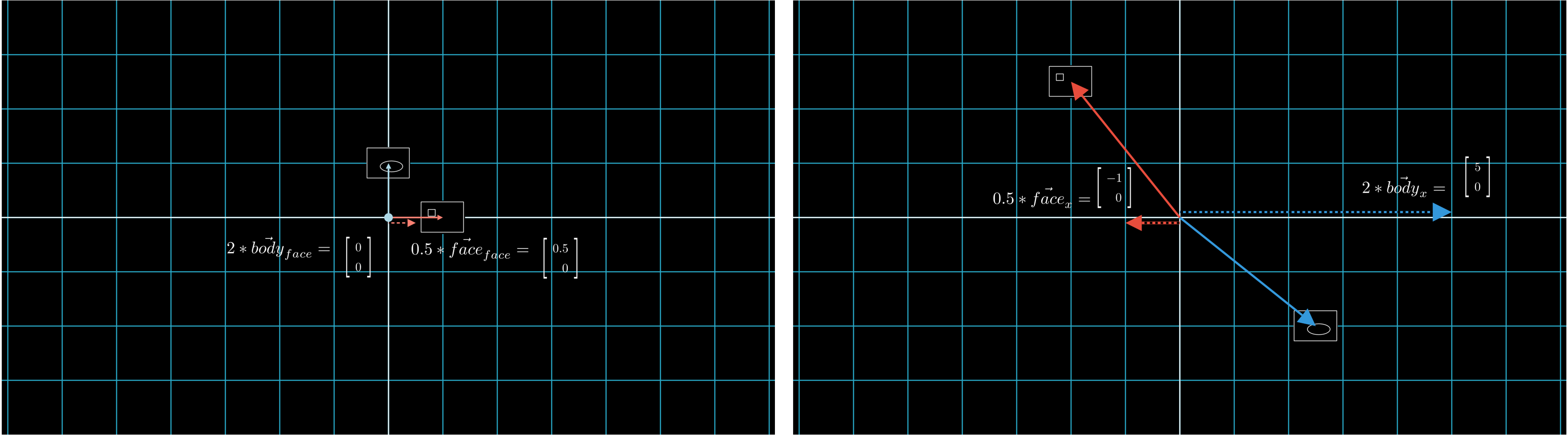
Next, we’re multiplying the first row of our matrix by the input vector:

$I$: $\def\a{\color{red}{1}} \def\b{\color{blue}{0}} \begin{bmatrix} \a & \b \end{bmatrix} \begin{bmatrix} 0.5 \\ 2 \end{bmatrix} -> \color{red}{1} * 0.5\qquad \color{blue}{0} * 2$

$W$: $\def\a{\color{red}{-2}} \def\b{\color{blue}{2.5}} \begin{bmatrix} \a & \b \end{bmatrix} \begin{bmatrix} 0.5 \\ 2 \end{bmatrix} -> \color{red}{-2} * 0.5\qquad \color{blue}{2.5} * 2$

[ STEP 3 ] Add: $\def\a{\color{red}{a}} \def\b{\color{blue}{b}} \begin{bmatrix} \a & \b \end{bmatrix} \begin{bmatrix} x_1 \\ x_2 \end{bmatrix} --> \color{red}{a} * x_{1} + \color{blue}{b} * x_2$

step3

Finally, we’ll finish the dot product by adding these terms together, obtaining the first element of our output vector:

$I$: $\def\a{\color{red}{1}} \def\b{\color{blue}{0}} \def\x{\color{purple}{0.5}} \begin{bmatrix} \a & \b \end{bmatrix} \begin{bmatrix} 0.5 \\ 2 \end{bmatrix} -> \color{red}{1} * 0.5 + \color{blue}{0} * 2 = \color{purple}{0.5} -> \begin{bmatrix} \x \\ ? \end{bmatrix} = X$

$W$: $\def\a{\color{red}{-2}} \def\b{\color{blue}{2.5}} \def\x{\color{purple}{4}} \begin{bmatrix} \a & \b \end{bmatrix} \begin{bmatrix} 0.5 \\ 2 \end{bmatrix} -> \color{red}{-2} * 0.5 + \color{blue}{2.5} * 2 = \color{purple}{4} -> \begin{bmatrix} \x \\ ? \end{bmatrix} = O$

If we apply the same logic of these three steps to row 2, we obtain the values of $O$, completing the main goal of this Chapter: ⁵

\[\def\x{\color{purple}{4}} \def\y{\color{purple}{-2.75}} O = \begin{bmatrix} \x \\ \y \end{bmatrix}\]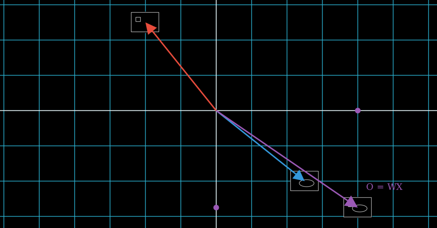

Neurons do NOT always Cleanly Correspond to a Human-Defined Concept

In our examples, for the purpose of gaining intuition, we defined our neurons, represented as basis vectors here, in terms of “human-understandable measurements”. For example, we can clearly understand what it means to measure body size, and have a vague understanding of what it means for an animal to be “more like a cat” than another animal. But neurons are not always “human-understandable”. In fact, most of the millions of neurons in many neural networks may not be. What may be is that each neuron does have a role in affecting the calculations of other neurons. For example, one neuron’s role may be to act as a “signal” for another neuron- if neuron A is low, neuron B will disregard information from neuron C because C must pass through A to get to B, and vice versa. This relationship between neurons has led to research such as finding neuron circuits ⁶. The true “roles” of neurons in spreading information to other neurons remains mysterious, and is still a subject of research.

We have finished going over the intuition behind matrix multiplication, which serves as the main operation behind not just neural networks, but in many methods of statistics and machine learning. In future Chapters, we will use this intuition to gain deep understandings of methods that use matrix multiplication to find new insights in data. The next Chapter will apply our new intuitive perceptions to controlling features in generative model outputs.

NEXT: CHAPTER 2.1

Note that the dot product between two vectors scales the numbers in the first vector, then adds them all together. The second vector contains the weights used to scale the first vector’s elements. Since the dot product is commutative, it is interchangable which vector is the “first” or “second”. ↩
The entity is neither 2 (meters) nor 6.56 (feet); those are just measurements labeling the data sample from two different perspectives. Remember, the dimensions are merely labels measuring the entity, but are not part of the entity itself. They are a way for an outside observer to describe the entity. So the vectors $X$ and $O$ are just different ways to measure the same data sample, but they are not the data sample itself. ↩
It is not hard to imagine that if we wanted to find the new values measuring MULTIPLE inputs, then instead of vector X, we use a matrix X, such that each column is a single input vector labeling a data sample. ↩
Remember that [1, 1.5] is NOT a basis vector, so is no longer labeled by a basis vector. ↩
We can gain further intuition about this by multiplying by the inverse of this matrix step-by-step; for instance, going down 2 rat units, and 1 cat, gets you to body size 1. ↩
See this link on Distill ↩