CHAPTER 2.1

CHAPTER 2.1: Changing Features using Vector Addition

(Reading time: 7 minutes)

Prerequisites: Chapter 1, what is a GAN ¹, and what is StyleGAN ²

StyleGAN is a generative model that was designed for more control over which features are outputted in an image. It was found that its latent space was very “disentangled”, meaning that one could have more control over one feature without affecting others ³.

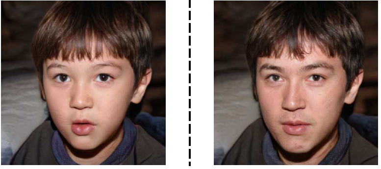
Let’s consider a scenario where we have an image outputted by StyleGAN, but we want to change one or more features of the image while keeping the other features the same. For example, in the picture below, we have an outputted image on the left. Then on the right, we have another outputted image where most of the features such as hair color and eye color are kept the same as the left image, while the age is changed.

**Image Source: Yujun Shen, Jinjin Gu, Xiaoou Tang, and Bolei Zhou. Interpreting the latent space of GANs for semantic face editing. CoRR, abs/1907.10786, 2019.**

Recall from Chapter 1 that features can be approximated as vectors in the latent space of neuron activations.

In the image above, the animal (a cat) is interpreted in terms of the features of Face Length and Body Size. For instance, by increasing the value of the “Body Size vector” on the y-axis from y=2 to y=3, we obtain a vector that is similar to the one mapped to the sample at (0.5, 2), but with a longer body. Given that the sample at (0.5, 2) represents an average cat, a sample at (0.5, 3) would represent a long cat.

When the feature we want to change is on the basis vector, all we have to do is change the value on the basis vector. But recall that features are not always on the basis vector; for instance, in the previous Chapter, we discussed a vector called “in terms of Cat”, shown in orange in the figure below. This vector was mapped to a feature that measured how much “like a Cat” a sample was. When the basis vectors were “Face Length” and “Body Size”, this vector “in terms of Cat” was not on the basis.

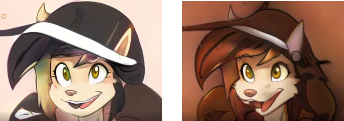
What if we had an image, say of a furry (an anthropomorphic animal-human hybrid cartoon), that originally had Cat features, but we want to increase these Cat features and make it more cat-like? For example, in the figure below, we would want to make the face on the left appear more animalistic, as on the right, while having the right image bear a resemblence to the one on the left in terms of features such as hair style, ears, smile, eye shape, skin tone, and more.

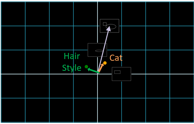
**These are actual outputs by a StyleGAN trained on images of furries.**

If we perform a Change of Basis to measure our image on the left in terms of “Cat”, then that would mean, in the second coordinate space, finding an image to the right of our image, with as little change in any other direction (such as Hair Style) as possible. Since Hair Style is measured on the y-axis, our second image should be as vertically aligned to the first image as much as possible. ⁴

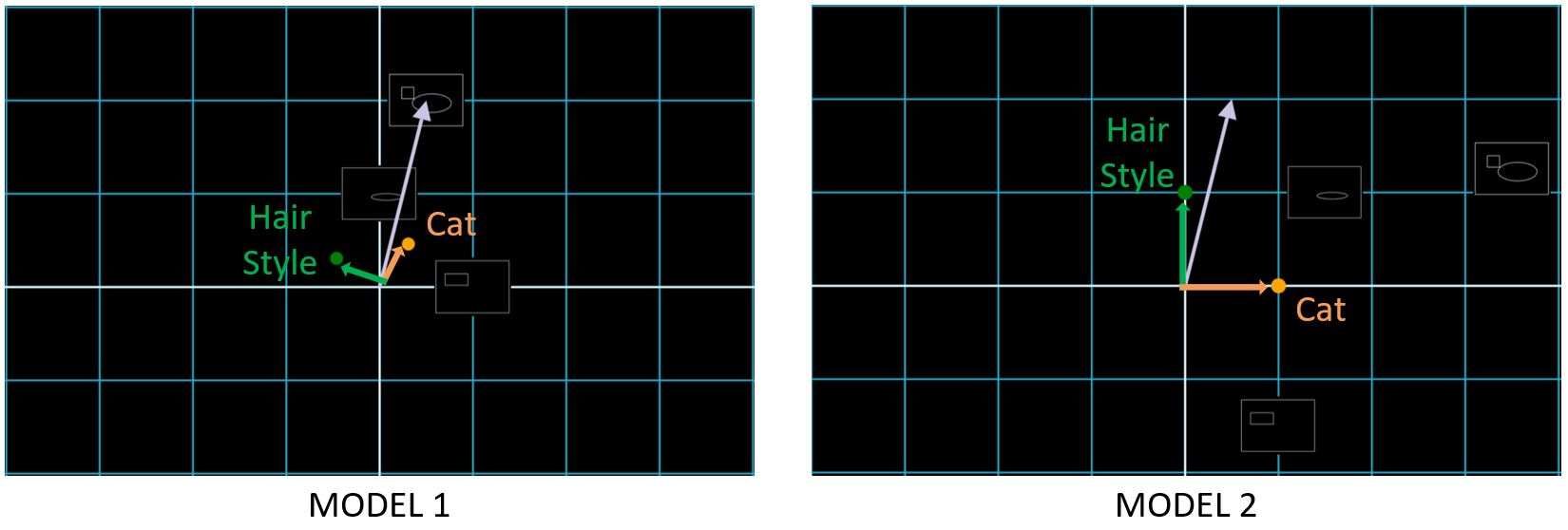
Note that when we move along the “Cat” vector but not along the “Hair Style” vector, we may still move along the “Ears” vector, demonstrating the difficulty of preserving as many features as possible while still deviating from one feature.

So if we only want to change one feature such as “cat-like”, we should “move along” that “cat-like” feature vector.

But how do we change the “Cat-like” feature while preserving (in other words, conditioning on) other features such as “Hair Style” or “Ear Style”?

One method to do this, called InterFaceGAN, was presented in the paper “Interpreting the Latent Space of GANs for Semantic Face Editing” ⁵. InterFaceGAN is now widely used approach for editing the features of StyleGAN generated images. In this Chapter, we’ll be explaining the intuition behind the mathematical calcuations used in InterFaceGAN.

Changing a Feature on the Basis Vector

First, let’s start with a simpler case, where the feature we want to change is on a basis vector. Say the Body Size vector is on the y-axis. We have a vector $z=[3,2]$ where Body Size = 2, and we want to find a similar vector, such as one where Body Size = 1. Since $y = [0,1]$, our feature vector Body Size is represented by $y$, so all we need to do is to add $y$ to $z$:

\[\vec{z} + \alpha * \vec{y}\] \[= \begin{bmatrix} 3 \\ 2 \end{bmatrix} + \alpha * \begin{bmatrix} 0 \\ 1 \end{bmatrix}\]

In which $\alpha$ is a scalar of any real number ⁶ that controls “how much” of Body Size $y$ is added.

Since vector addition adds the head of a vector with the tail of another vector, visually, this would look like:

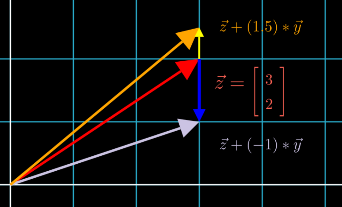
Such that the yellow and blue vectors represent $\alpha * \vec{y}$ being added to vector $z$.

Changing a Feature NOT on the Basis Vector

Next, let’s change a feature that’s not on the basis vector. Recall that a feature vector $n$ in a coordinate space is a measurement by the space’s basis vectors. In other words, each feature can be expressed entirely by a linear combination of basis vectors. So if feature $n$ represents “cat-like”, then how much a sample is like a cat is represented by its combination of Face Length to Body Size.

(Click on the following optional section to expand it. It is optional reading as the validity of its interpretation is still up for questioning.)

Features and Gradients:

In the case of using basis vectors as measurements, the entire line represented "how much" of a quantity there was.

In this case, the neural network has learned that a "typical" cat would have a Face Length of 0.5 and a Body Size of 2 (it learned to use this ratio to distinguish a cat from other animals in its dataset), so the ratio of Body Length to Face Length is 2:0.5, or 4. If a sample it sees has this ratio of around 4, it is "likely to be a cat". Ratios are relative, so even if we have absolute units of Body Length = 8 and Face Length = 2, the ratio 8:2 = 4 indicates to the neural network that this sample is more likely a cat than any other animal.

As taught in algebra, this is the slope of a line, where "rise/run" in this case means "Body Length / Face Length". But vectors do not have slopes; only functions have slopes, and lines are functions. It seems that the vectors that lie on the line with this slope all correspond to some feature.

Essentially, each feature is mapped to a line's steepness and direction, or its angle from the origin of basis vectors, and stretching or shrinking a vector would alter its magnitude, and thus "how much" of that feature there is.

Note that in higher dimensional spaces, instead of describing this ratio as "rise/run", it is better to use "steepness and direction" instead. You can say this is the gradient in gradient descent, in which how each neuron measures the data is changed according to the gradient. The vector is both an "object" measuring a feature, and a "relation" determining how a feature is used to change another feature.

How features relate to functions and their gradients is still unclear, and remains a subject of further investigation.

Similar to the example we showed where the feature is on the basis vector, we want to “add” feature n to z. What does this actually mean?

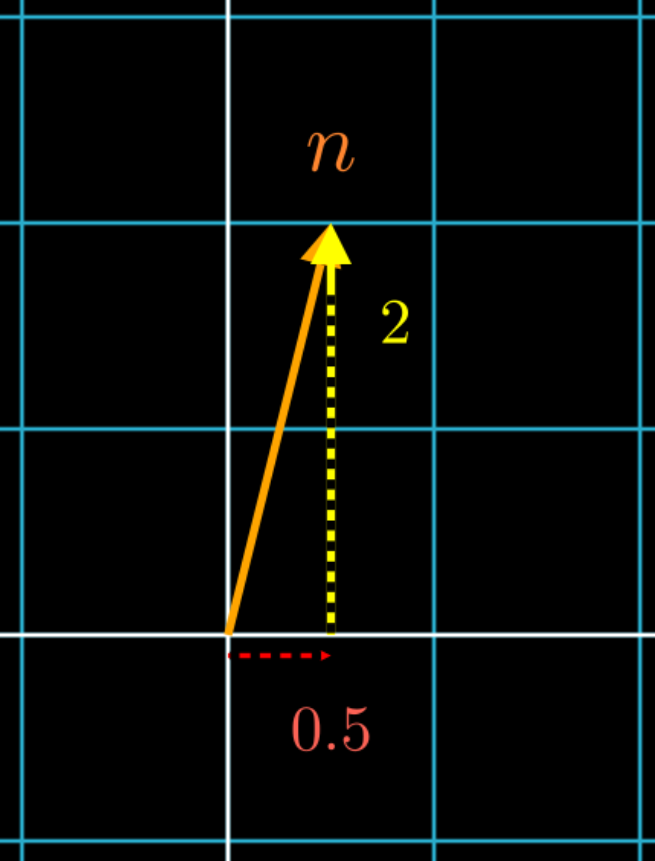
In the previous example, all we had to do to change $z$ by $y$ was $\vec{z} + \alpha * \vec{y}$, because the feature on $y$ did not require any units of $x$ to be represented. But now, the feature cat is represented by vector $n$ using BOTH units of $x$ and $y$. So instead of just adding $y$, we have to add both $x$ and $y$:

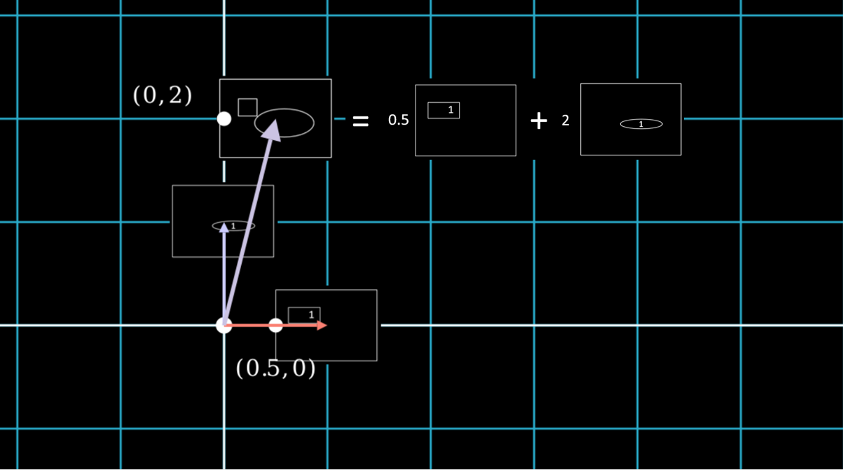
\[\vec{z} + \alpha * (0.5 * \vec{x} + 2 * \vec{y})\]

Since feature cat is $\vec{n} = 0.5 * \vec{x} + 2 * \vec{y}$, this linear combination can be rewritten as:

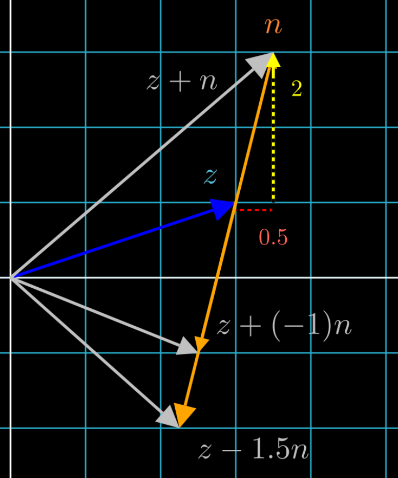
\[\vec{z} + \alpha * \vec{n}\]

Visually, this would look like the figure below, in which will get to the same point whether you follow the red then yellow vectors $(0.5 * \vec{x} + 2 * \vec{y})$, or just the orange vector $(\vec{n})$:

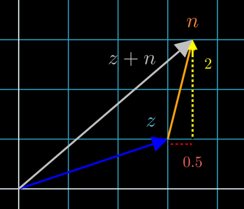
Using $\alpha$, we can add or subtract as many units of “cat” to z as we like.

At first, it’s not obvious how we “change z by n cat units”. So let’s perform a change of basis where the cat feature is mapped to a basis vector, to truly show how each sample is measured in cats:⁷

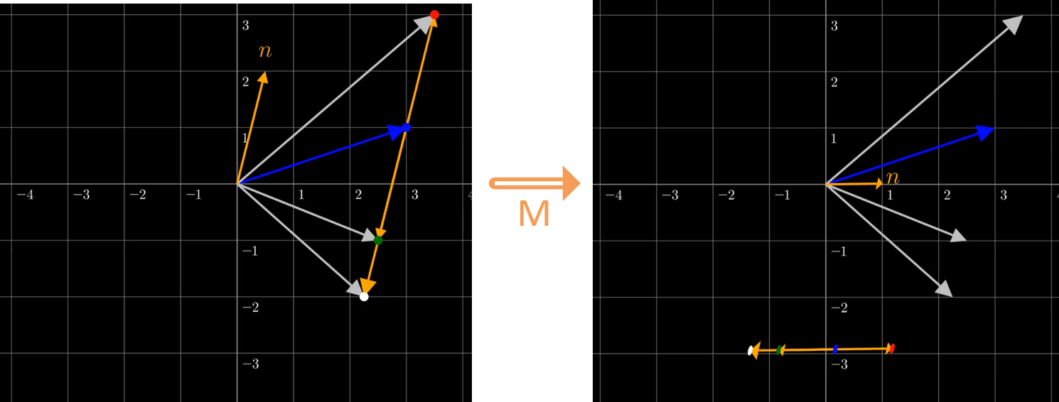
Each sample, shown as dots in the figure, can be interpreted as having “units of cat”, shown in orange. The red dot, originally on $\vec{z} + (1)\vec{n}$, is close to having “1” cat unit. The blue dot, originally on $\vec{z} + (0)\vec{n}$, is close to having “0” cat units. The same goes for the green and white dots, having -1 and -1.5 cat units, respectively. We see that the number of cat units corresponds to $\alpha$ in the equation $\vec{z} + \alpha * \vec{n}$.⁸ Also note how $\vec{n}$ and the line containing $\vec{z} + \alpha * \vec{n}$ are parallel.

We can get better intuition of this when it’s animated:

Click here to see the video

What was the matrix $M$ used to perform this change of basis? Recall that each column of a matrix is a coordinate where features on basis vectors are sent to. So to send a feature on $[1,0]$ to $[0.5, 2]$, we would use the matrix:

$$ W = \begin{bmatrix} 0.5 & ? \\ 2 & ? \end{bmatrix} $$

Note that we have stated what will be sent to one basis vector; but in 2D coordinate space, there are two, so let’s find where to send the second one. To avoid too many changes in the coordinate space, let’s use a rotation matrix. A rotation matrix requires that both column vectors are at 90 degree angles, so we’ll use a technique to find a vector that’s 90 degrees to [0.5, 2]. Then this rotation matrix is:

$$ W = \begin{bmatrix} 0.5 & -1 \\ 2 & -0.25 \end{bmatrix} $$

However, this is NOT the matrix $M$ we use to perform the change of basis above. We don’t want to send a basis vector to a certain coordinate; we want to do the opposite, where we send a feature from a coordinate to a basis vector. So we have to take the inverse of the matrix in order to send the cat feature from $[0.5, 2]$ to $[1, 0]$. The inverse of the matrix above, rounded to 4 decimal places, is:

$$ M = W^{-1} = \begin{bmatrix} -0.1333 & 0.5333 \\ -1.0667 & 0.2667 \end{bmatrix} $$

This is the matrix $M$ we use to perform the change of basis in the example above.

In the example above, note how each sample has different values of n, but all have the same value (close to -3) along the 2nd basis vector. Why are the values along this 2nd basis vector, which is mapped to a feature that is 90 degrees to the cat feature vector, preserved after $\vec{z} + \alpha * \vec{n}$? We’ll find out why in the next section.

NEXT: CHAPTER 2.2

In this section, all that’s needed to know is that a GAN takes a latent vector z from a latent space- that is, a space that represents features much like the latent space of activations we discussed in Chapter 1- and outputs an image. Other concepts from GANs can enhance the connections made as this chapter is studied, but are not required. A review of GANs can be found here. ↩
In this section, all you have to know is that StyleGAN is a type of generative model (a neural network that outputs an image). A deeper understanding of StyleGAN can enhance the connections made as this chapter is studied, but are not required. A quick explanation of StyleGAN can be found here ↩
https://paperswithcode.com/paper/stylespace-analysis-disentangled-controls-for ↩
This is similar to the example in the previous Chapter, but instead of changing to a basis where “like a Rat” is mapped to the y-axis, the feature “Hair Style” is mapped to the y-axis. ↩
Yujun Shen, Jinjin Gu, Xiaoou Tang, and Bolei Zhou. Interpreting the latent space of GANs for semantic face editing. CoRR, abs/1907.10786, 2019. ↩
In a simplified definition, a real number is allowed to be a fraction, negative, irrational, but not imaginary. See: https://en.wikipedia.org/wiki/Real_number ↩
Here, we do not change the silver and blue vectors, but change the orange vectors, because the orange vectors represent “cat units”. This goes against the idea in Chapter 1 that “vectors stay, but data points change”, in which the vectors are mapped to data points. However, here we do change the vectors only for intuitive purposes, as it shows how the cat vector now acts as a measurement along the basis vector. This is just an informal way to explain intuition; the idea that “vectors stay, but data points change” remains. ↩
Each one may only be “close” to the number of cat units due to the decimal point approximations used in the matrix to represent the actual values. ↩